On this page, you will find more information about the rare biosphere present in our greenhouse samples.

How We Chose Our Rare Bioshphere

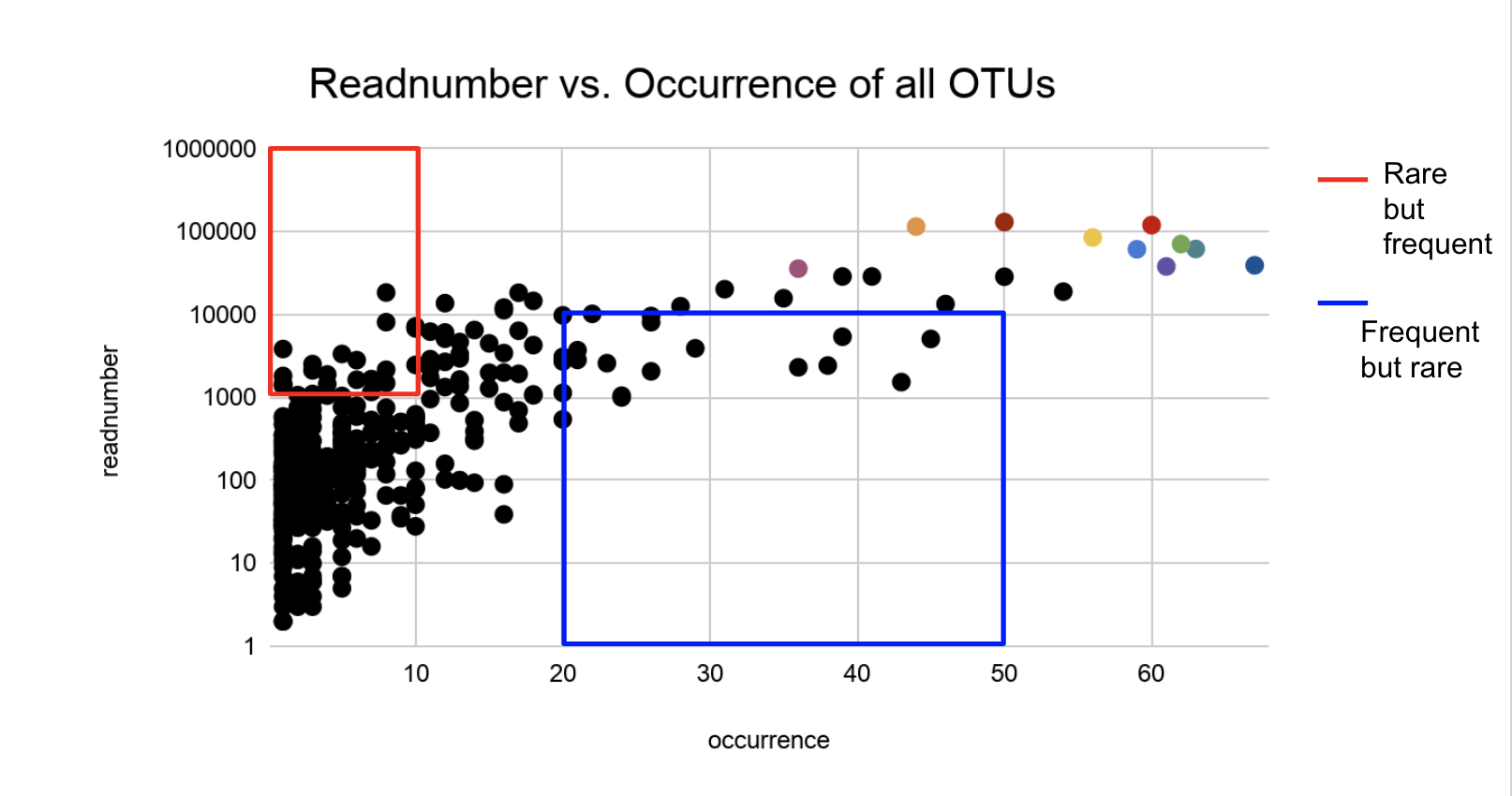
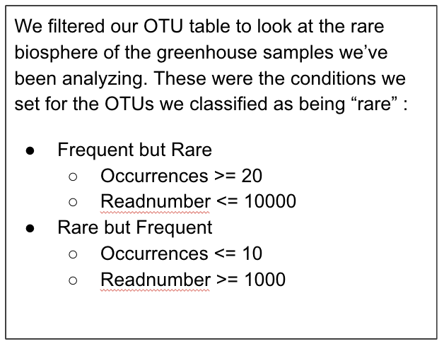
Frequent but Rare OTUs

Figure 1: SAR Composition of Frequent but Rare OTUs

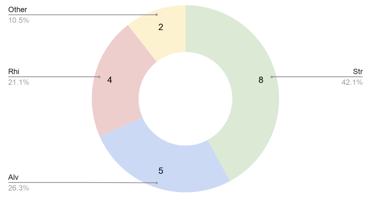
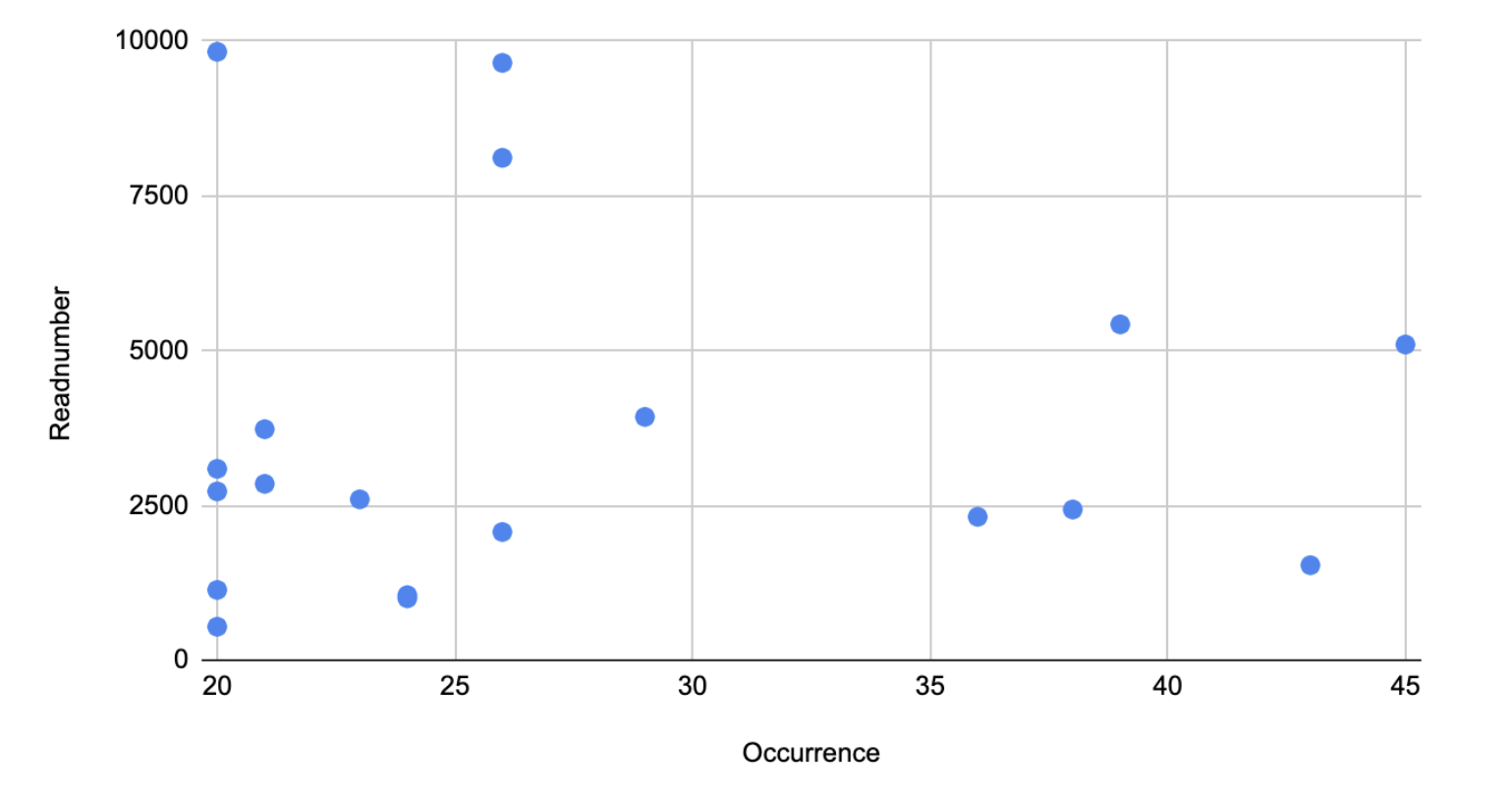
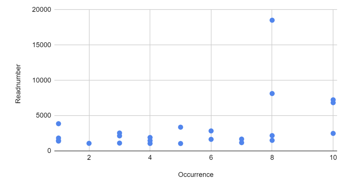
After filtering our spreadsheet to keep OTUs that were frequent but rare, we ended up with a total of 19 out of 407 OTUs. These 19 OTUs, were mostly composed of stramenopiles. The “Other” category in this plot represents possible contaminants in our data.

Figure 2: Readnumber vs Occurrence (Frequent but Rare)

This is a closer look at the blue box: the occurrence and readnumber of each of our samples considered frequent but rare (readnumbers less than or equal to 10,000 and occurrences less than or equal to 50).

Frequent but Rare OTU Table

Frequent_but_Rare <- read.csv("Frequent but Rare.csv")
print(Frequent_but_Rare)

##       OTU Likely.organism   SAR
## 1   OTU48            alga   Str
## 2   OTU51         ciliate   Alv
## 3   OTU77  testate amoeba   Rhi
## 4  OTU114       cercozoan   Rhi
## 5   OTU75       oomycetes   Str
## 6   OTU73          diatom   Str
## 7   OTU87         ciliate   Alv
## 8   OTU94         ciliate   Alv
## 9   OTU76    contaminant? Other
## 10 OTU105    contaminant? Other
## 11  OTU88         ciliate   Alv
## 12 OTU143       cercozoan   Rhi
## 13 OTU127      flagellate   Str
## 14  OTU58      falgellate   Str
## 15  OTU80       cercozoan   Rhi
## 16 OTU150         ciliate   Alv
## 17 OTU173        oomycete   Str
## 18 OTU163        oomycete   Str
## 19 OTU369          diatom   Str

This table, shows the likely organism these 19 OTUs are when we blasted them using the National Center of Biotechnology Information (NCBI) services, specifically, the Basic Local Alignment Search Tool (BLAST). ¹

Rare but Frequent OTUs

Figure 1: SAR Composition of Rare but Frequent OTUs

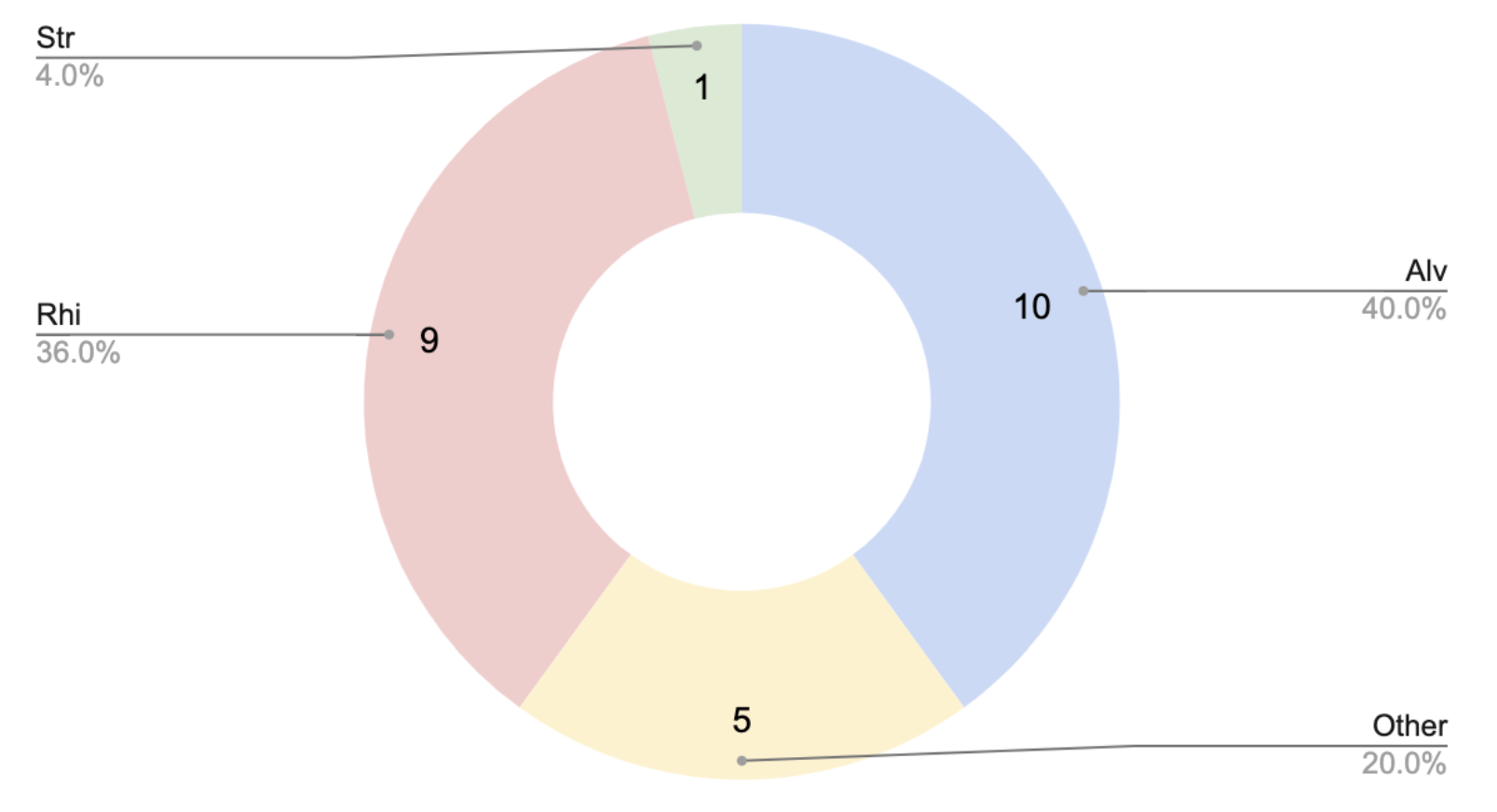
After filtering our spreadsheet to keep OTUs that were rare but frequent, we ended up with a total of 25 OTUs. Most of the rare but frequent OTUs are heterotrophs within rhizaria and alveolata. The “other” category is possible contaminants.

Figure 2: Readnumber vs Occurrence (Rare but Frequent)

This is a closer look at the previous red box depicting the occurrence and readnumber of our rare but frequent OTUs (readnumbers greater than or equal to 1000 and occurrences less than or equal to 10). Most of these frequent OTUs have below 5000 reads, but one OTU stands out: OTU43 with an occurrence of 8 and 18518 reads. It is a testate amoeba within rhizaria.

Rare but Frequent OTU Table

Rare_but_Frequent <- read.csv("Rare but Frequent.csv")
print(Rare_but_Frequent)

##       OTU Likely.organism   SAR
## 1  OTU118        Ciliate    Alv
## 2  OTU136        Ciliate    Alv
## 3   OTU63    contaminant? Other
## 4  OTU179        Ciliate    Alv
## 5  OTU181       Heliozoan   Rhi
## 6  OTU106    contaminant? Other
## 7   OTU52       Cercozoan   Rhi
## 8   OTU74       Cercozoan   Rhi
## 9  OTU237        Ciliate    Alv
## 10 OTU113        Ciliate    Alv
## 11 OTU177  Testate Amoeba   Rhi
## 12 OTU165    Golden Algae   Str
## 13  OTU99       Euglyphid   Rhi
## 14 OTU104       Cercozoan   Rhi
## 15  OTU92        Ciliate    Alv
## 16 OTU123        Ciliate    Alv
## 17 OTU164        Ciliate    Alv
## 18 OTU157        Ciliate    Alv
## 19  OTU43  Testate Amoeba   Rhi
## 20  OTU45      Flagellate   Rhi
## 21 OTU128        Ciliate    Alv
## 22 OTU221    contaminant? Other
## 23  OTU78       Cercozoan   Rhi
## 24  OTU47    contaminant? Other
## 25 OTU130    contaminant? Other

This table, shows the likely organism these 25 OTUs are when we blasted them using the National Center of Biotechnology Information (NCBI) services, specifically, the Basic Local Alignment Search Tool (BLAST).²

Diversity Indices/Rarefaction Curves

Figure 1: Rarefaction Curve of Observed OTUs

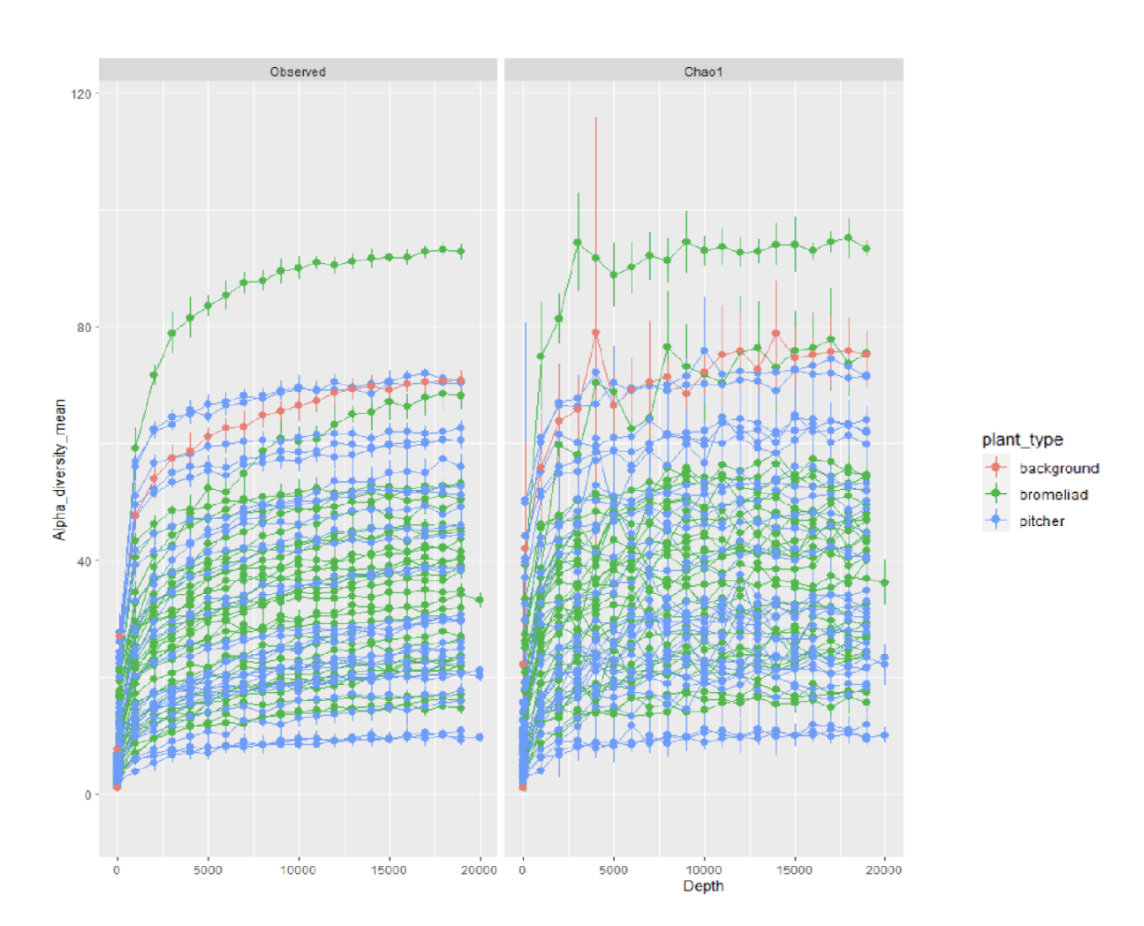
This is a rarefaction curve with 20,000 reads, colored by plant type. The observed number of OTUs for a certain number of reads are on the left and the Chao1 calculations, which consider the rare biosphere, are on the right. The top bromeliad sample stands out in its diversity. The background sample, in red, also.

Figure 2: Richness Plot of Observed OTUs

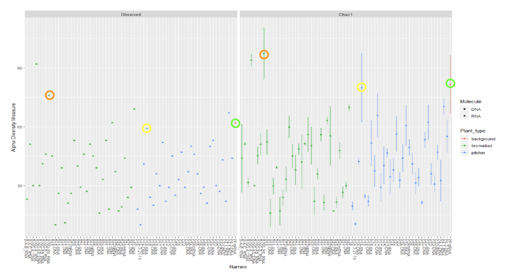
This is a richness plot of the observed OTUs within the samples vs. the Chao1 estimates. Pitcher samples (green) on the left do not have a distinct pattern from the bromeliad samples (blue) on the right, but there are some samples, including the background sample (red) that have much higher Chao1 estimates (indicating a diverse rare biosphere) than observed values (circled in colored pairs).

Chunk of code used to make richness plot.

plot_richness(merged_physeq, x = "Names", color = "Plant_type", shape = "Molecule",
title = NULL, scales = "fix", nrow = 1, shsi = NULL,
measures = c("Observed", "Chao1"), sortby = NULL)

All figures and tables presented on this website were made by Jailene and Hannah using R/RStudio, Google Sheets, Procreate, and Microsoft Excel.

Rare Biosphere

Jailene Gonzalez and Hannah Rappaport

Last updated on 2020-07-31